Community Detection and Model Selection for SBMs

### Community Detection and Model Selection in SBMs

![:scale 50%](images/neurodata_blue.png)

Eric W. Bridgeford         | {Biostatistics, BME, CIS}<br>
[ericwb95@gmail.com](mailto:ericwb95 at gmail dot com) 
| <https://neurodata.io/talks/commdetect.html>

---
name:talk

### Outline

- [Background](#back)
- [SBMs](#sbm)
- [Community Detection](#commdetect)
- [Model Selection](#modselect)

---
name:back

### Outline

- Background
- [SBMs](#sbm)
- [Community Detection](#commdetect)
- [Model Selection](#modselect)

---

### Background readings

- [Chapter 4 -- Network basics](https://docs.neurodata.io/graph-stats-book/representations/ch4/ch4.html)
- [Chapter 5.2 -- SBMs](https://docs.neurodata.io/graph-stats-book/representations/ch5/single-network-models_SBM.html)
- [Chapter 5.3 -- RDPGs](https://docs.neurodata.io/graph-stats-book/representations/ch5/single-network-models_RDPG.html)
- [Chapter 6.1 -- SBM estimation](https://docs.neurodata.io/graph-stats-book/representations/ch6/estimating-parameters_mle.html)
- [Chapter 6.4 -- RDPG estimation](https://docs.neurodata.io/graph-stats-book/representations/ch6/estimating-parameters_spectral.html)

---

name:sbm

### Outline

- [Background](#back)
- SBMs
- [Community Detection](#commdetect)
- [Model Selection](#modselect)

---

### SBM

- The nodes will represent regions of the brain (70)
- The edges will represent whether two regions are connected or not by a diffusion fiber tract
- The community membership vector $\vec z$ indicate which hemisphere (R/L) each node is in
- Block matrix $B$ has entries of $0.5$ for the L/L and R/R entries
  - $0.2$ for the R/L and L/R entries

---

### Defining the parameters of an SBM

```python
# import graspologic package
import graspologic as gp
```

```python
# set the number of nodes per hemisphere
nl = 35; nr = 35
ns = [nl, nr]

# the block matrix
B = [[0.5, 0.2], [0.2, 0.5]] # the block matrix

# the hemisphere of each node
zvec = ["L" for i in range(0, nl)] + ["R" for i in range(0, nr)]
# one-hot-encode node communities
zvec_ohe = np.vstack([[1,0] for i in range(0, nl)] + 
                    [[0, 1] for i in range(0, nr)])
# the probability matrix
P = zvec_ohe @ B @ zvec_ohe.transpose()
```

```python
fig, axs = plt.subplots(1,2, figsize=(15,6))
    
gp.plot.heatmap(np.array(B), ax=axs[0], title="Block Matrix", 
                xticklabels=["L", "R"], yticklabels=["L", "R"],
                cbar=False, annot=True)
gp.plot.heatmap(P, ax=axs[1], inner_hier_labels=zvec,
                title="Probability Matrix")
```

---

### Defining the Parameters of an SBM

<center>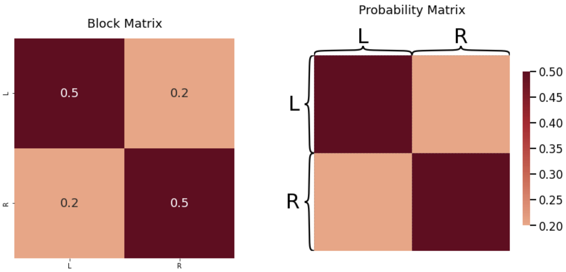
![:scale 100%](images/workshop/parameters.png)
</center>

---

### Simulating an SBM

```python
# simulate an adjacency matrix
A = gp.simulations.sbm(ns, B, directed=False, loops=False)

# ...and plot it
fig, axs = plt.subplots(1,2, figsize=(15,6))
    
gp.plot.heatmap(A, ax=axs[0], inner_hier_labels=zvec,
                title="$SBM_{70}(\\vec z, B)$ simulation")
gp.plot.heatmap(P, ax=axs[1], inner_hier_labels=zvec,
                title="Probability Matrix")
```

---

#### The community structure is totally obvious...

<center>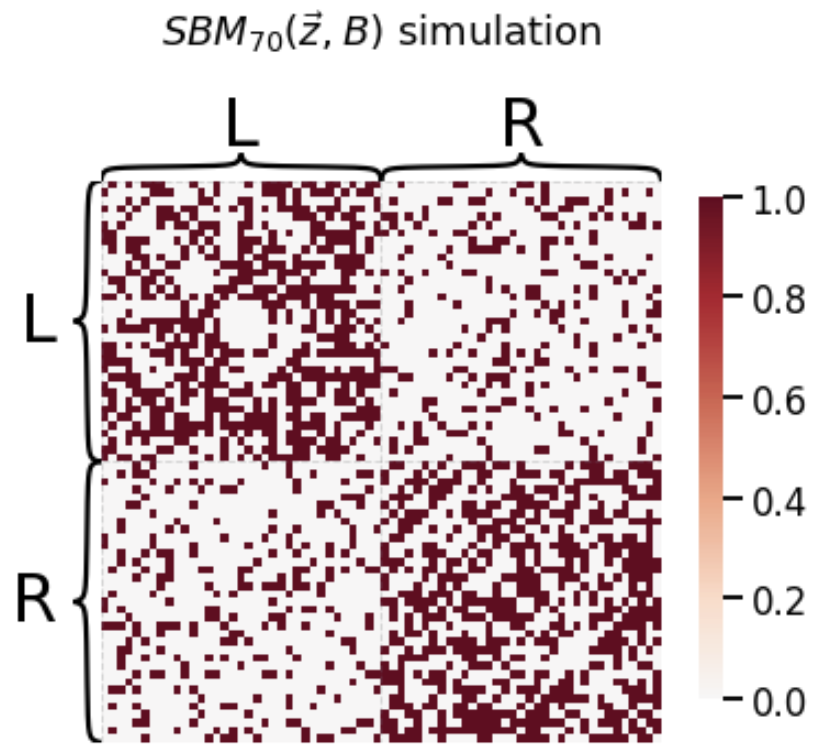
![:scale 60%](images/workshop/sbm.png)
</center>

---

### ... so why do we care?

- the community structure is .ye[only]  obvious for an ordering of the nodes in community order
  - we don't know community ahead of time

```python
import numpy as np
# generate a reordering of the n nodes
vtx_perm = np.random.choice(np.sum(ns), size=np.sum(ns), replace=False)
Aperm = A[tuple([vtx_perm])] [:,vtx_perm]
```

```python
gp.plot.heatmap(Aperm, title="$SBM_{70}(\\vec z, B)$, random node order")
```

---

### ... so why do we care?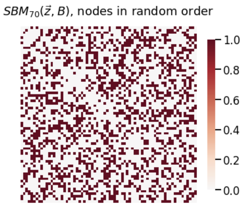

![:scale 60%](images/workshop/sbm_rand.png)

---

name:commdetect

### Outline

- [Background](#back)
- [SBMs](#sbm)
- Community Detection
- [Model Selection](#modselect)

---

### How do we "guess" community structure?

- Community detection: identifying unknown community labels
- Idea: nodes sharing a community tend to be connected to similar nodes
  - why? block matrix
  - probability matrix is "low rank": only need one vector per community
  - if network has $K$ communities, $P$ is rank-$K$

---

### What do we mean by "low-rank"?

- probability matrix only has two unique row/column vectors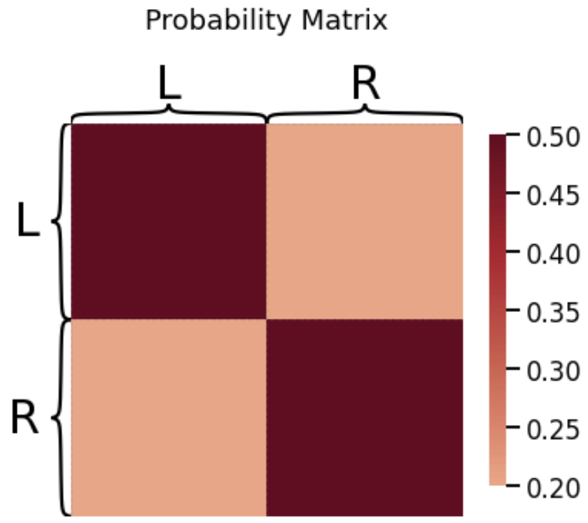

![:scale 60%](images/workshop/probmtx.png)

---

### How do we "guess" low-rank structure?

- when we have a low-rank structure, a way to deduce this structure is a spectral embedding
  - PCA but on a "similarity" matrix
    - in what sense were the nodes of the same community similar?

![:scale 40%](images/workshop/probmtx.png)
--

- probability, so we use the probability matrix

---

### How do we "guess" low-rank structure?

```python
# diagonal augmentation of the probability matrix
Paug = gp.utils.augment_diagonal(P)
# embed using spectral embedding
U, s, _ = np.linalg.svd(Paug)
Pembed = U[:,0:2] @ np.diag(s[0:2])
```

```python
import seaborn as sns

fig, ax = plt.subplots(1,1, figsize=(6,6))
sns.heatmap(Pembed, ax=ax)
```

---
### How do we "guess" low-rank structure?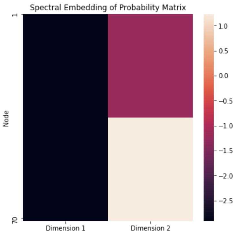

![:scale 60%](images/workshop/probmtx_embed.png)

---

### Finding a surrogate for the probability matrix

- Problem: we don't know the probability matrix ahead of time
  - we never know the "true" underlying statistical model
  - what can we use?
--

- it turns out that the adjacency matrix works well as a surrogate
  - ASE: .ye[A]djacency .ye[S]pectral .ye[E]mbedding

```python
ase = gp.embed.AdjacencySpectralEmbed()
Aembed = ase.fit_transform(A)
```

---

### How do we actually deduce community labels?

```python
fig, ax = plt.subplots(1,1, figsize=(6,6))
sns.heatmap(Aembed, ax=ax)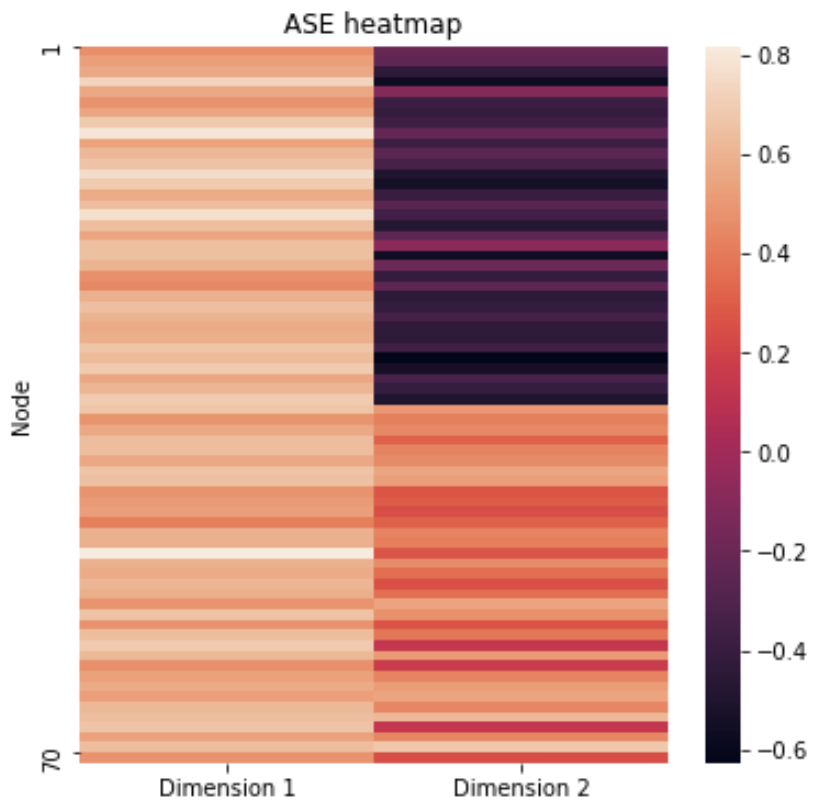
```

![:scale 40%](images/workshop/ase_heatmap.png)

---

### How do we actually deduce community labels?

```python
gp.plot.pairplot(Aembed, labels=zvec, legend_name="Community (Unknown)",
                 title="ASE Pairplot")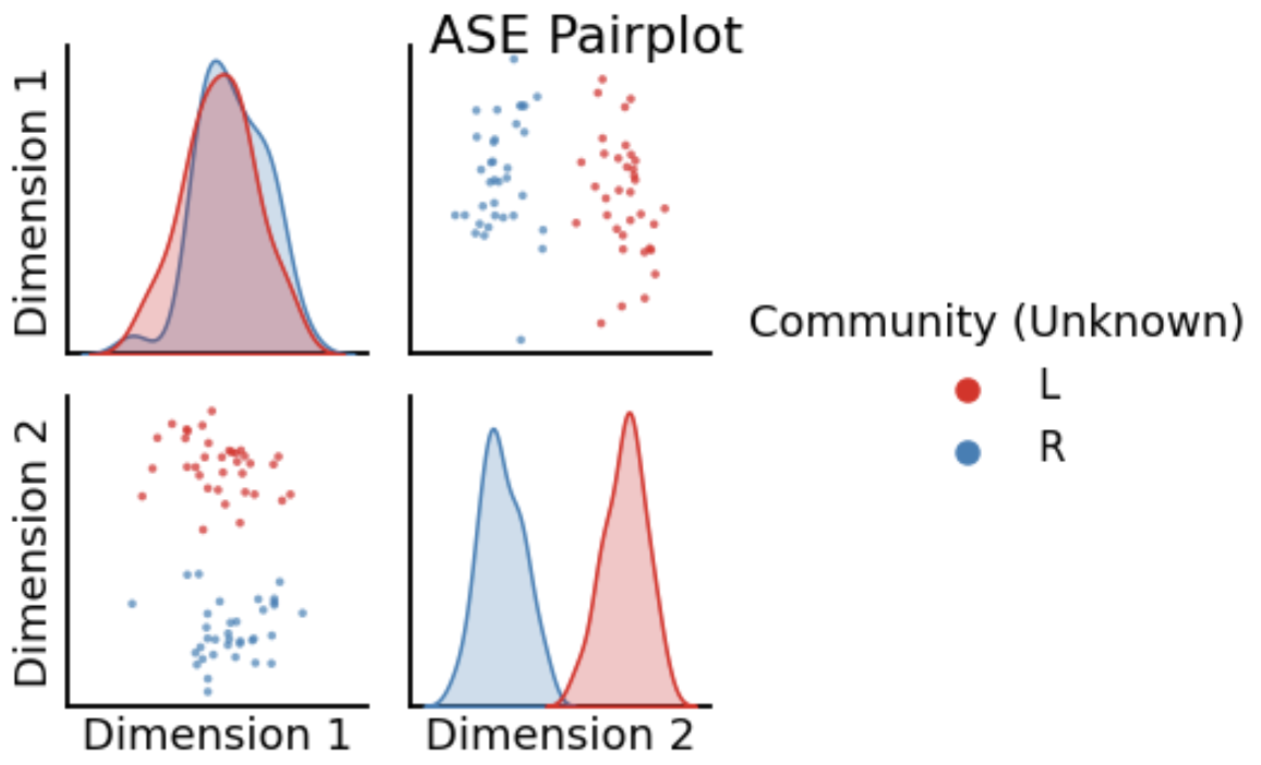
```

![:scale 80%](images/workshop/ase_pairplot.png)

---

### Community Detection

- take the ASE and cluster it
  - number of clusters = number of communities you expect
--

- evaluation: choose a metric which is high for "good" clusterings, and "low" for bad clusterings
  - Kmeans: ARI (.ye[A]djusted .ye[R]and .ye[I]ndex)

```python
from sklearn.cluster import KMeans
from sklearn.metrics import adjusted_rand_score

labels_kmeans = KMeans(n_clusters = 2).fit_predict(Aembed)
ari_kmeans = adjusted_rand_score(labels_kmeans, zvec)
```

---

### Evaluation of ASE

```python
gp.plot.pairplot(Aembed, labels=labels_kmeans, legend_name="Predicted",
                 title="ASE Pairplot (ARI={:.2f})".format(ari_kmeans))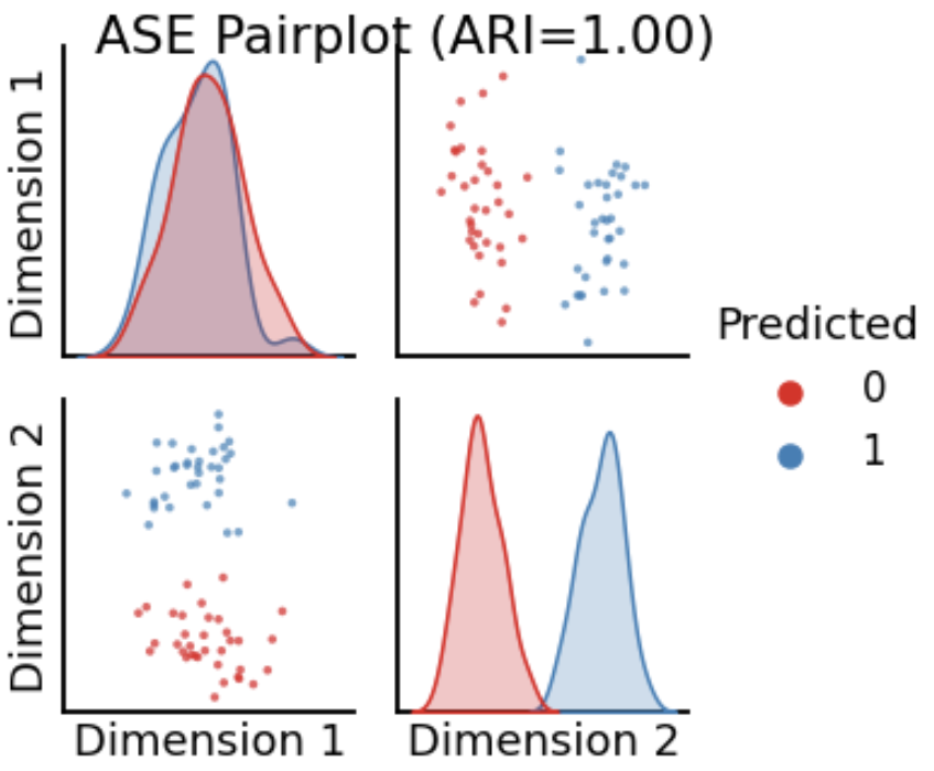
```

![:scale 70%](images/workshop/ase_pairplot_pred.png)

---

### Evaluation of ASE

- clustering is unsupervised: which cluster is Left vs. Right for examining error rate?
- `gp.utils.remap_labels()`: "rename" (0/1 to Left/Right) labels of the unsupervised predictions 
  - as many samples as possible have the same label in unsupervised predictions and the true labels

```python
# remap with graspologic
labels_kmeans_remap = gp.utils.remap_labels(zvec, labels_kmeans.astype(str))

# errors are where the prediction != the true label
error = zvec != labels_kmeans_remap
# error rate is the frequency of making an error
er_rt = np.mean(error)

palette = {'Right':(0,0.7,0.2),
           'Wrong':(0.8,0.1,0.1)}

# initialize numpy array for each node
error_label = np.array(len(zvec)*['Right'])
# add label 'Wrong' for each error that is made
error_label[error] = '›'
```

---

### Evaluation of ASE

```python
gp.plot.pairplot(Aembed, labels=labels_kmeans_remap, legend_name="Predicted",
                 title="ASE Pairplot (ARI={:.2f})".format(ari_kmeans))
```

![:scale 70%](images/workshop/ase_pairplot_pred_rename.png)

---

### Evaluation of ASE

```python
gp.plot.pairplot(Aembed, labels=error_label,
                 legend_name="Prediction successful?",
                 title="ASE Pairplot (Error={:.2f})".format(er_rt), 
                 palette=palette)
```

![:scale 70%](images/workshop/ase_pairplot_er.png)

---

### How do we decide the number of communities?

- If we don't know the number of communities ahead of time, what do we do?

--
- use a performance metric!
  - a good choice tends to be the Silhouette score
  - clusterings with high Silhouette $\Rightarrow$ better
  - clusterings with low Silhouette $\Rightarrow$ worse
--

- repeat clustering for "plausible" numbers of clusters, and pick the one where Silhouette is highest

```python
from pandas import DataFrame as df

comm_select = gp.cluster.KMeansCluster(max_clusters=10)
comm_select = comm_select.fit(Aembed)
nclusters = range(2, 10)
silhouette = comm_select.silhouette_

silhouette_df = df({"Number of Clusters": nclusters,
                    "Silhouette Score": silhouette})
```

---

### How do we decide the number of communities?

```python
fig, ax = plt.subplots(1,1,figsize=(7, 4))

sns.lineplot(data=silhouette_df,ax=ax, x="Number of Clusters",
             y="Silhouette Score");
ax.set_title("Silhouette Analysis of KMeans Clusterings")
ax.set_ylim([-1, 1])
```

![:scale 70%](images/workshop/silhouette.png)

---

name:modselect

### Outline

- [Background](#back)
- [SBMs](#sbm)
- [Community Detection](#commdetect)
- Model Selection

---

### Links

- [Graspologic python package](https://github.com/microsoft/graspologic)
- [Graspologic book repository](https://github.com/neurodata/graph-stats-book)
- [Graspologic book](http://docs.neurodata.io/graph-stats-book/coverpage.html)
- Questions?